Languageen
planetary-computer-reading-stac.ipynb

Reading Data from the STAC API

The Planetary Computer catalogs the datasets we host using the STAC (SpatioTemporal Asset Catalog) specification. We provide a STAC API endpoint that can be used to search our datasets by space, time, and more. This quickstart will show you how to search for data using our STAC API and open-source Python libraries. For more on how to use our STAC API from R, see Reading data from the STAC API with R.

To get started you'll need the pystac-client library installed. You can install it via pip:

> pip install pystac-client

First we'll use pystac-client to open up our STAC API:

In [1]:
from pystac_client import Client

catalog = Client.open("https://planetarycomputer.microsoft.com/api/stac/v1")

Searching

We can use the STAC API to search for assets meeting some criteria. This might include the date and time the asset covers, is spatial extent, or any other property captured in the STAC item's metadata.

In this example we'll search for imagery from Landsat Collection 2 Level-2 area around Microsoft's main campus in December of 2020.

In [2]:
time_range = "2020-12-01/2020-12-31"
bbox = [-122.2751, 47.5469, -121.9613, 47.7458]

search = catalog.search(collections=["landsat-8-c2-l2"], bbox=bbox, datetime=time_range)
items = search.get_all_items()
len(items)
Out[2]:
4

In that example our spatial query used a bounding box with a bbox. Alternatively, you can pass a GeoJSON object as intersects

area_of_interest = {
    "type": "Polygon",
    "coordinates": [
        [
            [-122.2751, 47.5469],
            [-121.9613, 47.9613],
            [-121.9613, 47.9613],
            [-122.2751, 47.9613],
            [-122.2751, 47.5469],
        ]
    ],
}

time_range = "2020-12-01/2020-12-31"

search = catalog.search(
    collections=["landsat-8-c2-l2"], intersects=area_of_interest, datetime=time_range
)

items is a pystac.ItemCollection. We can see that 4 items matched our search criteria.

In [3]:
len(items)
Out[3]:
4

Each pystac.Item in this ItemCollection includes all the metadata for that scene. STAC Items are GeoJSON features, and so can be loaded by libraries like geopandas.

In [4]:
import geopandas

df = geopandas.GeoDataFrame.from_features(items.to_dict(), crs="epsg:4326")
df
Out[4]:
geometry datetime platform proj:bbox proj:epsg description instruments eo:cloud_cover view:off_nadir landsat:wrs_row landsat:scene_id landsat:wrs_path landsat:wrs_type view:sun_azimuth view:sun_elevation landsat:cloud_cover_land landsat:processing_level landsat:collection_number landsat:collection_category
0 POLYGON ((-122.74802 48.51223, -120.22983 48.0... 2020-12-29T18:55:56.738265Z landsat-8 [471585.0, 5136885.0, 705015.0, 5373315.0] 32610 Landsat Collection 2 Level-2 Surface Reflectan... [oli, tirs] 100.00 0 027 LC80460272020364LGN00 046 2 162.253231 17.458298 100.00 L2SP 02 T2
1 POLYGON ((-124.29833 48.51325, -121.79248 48.0... 2020-12-20T19:02:09.878796Z landsat-8 [353385.0, 5135085.0, 589215.0, 5374215.0] 32610 Landsat Collection 2 Level-2 Surface Reflectan... [oli, tirs] 100.00 0 027 LC80470272020355LGN00 047 2 163.360118 17.414441 100.00 L2SP 02 T2
2 POLYGON ((-122.75189 48.51190, -120.23406 48.0... 2020-12-13T18:56:00.096447Z landsat-8 [471285.0, 5136885.0, 704715.0, 5373315.0] 32610 Landsat Collection 2 Level-2 Surface Reflectan... [oli, tirs] 98.73 0 027 LC80460272020348LGN00 046 2 164.126188 17.799744 98.64 L2SP 02 T2
3 POLYGON ((-124.29534 48.51347, -121.78981 48.0... 2020-12-04T19:02:11.194486Z landsat-8 [353685.0, 5135085.0, 589515.0, 5374215.0] 32610 Landsat Collection 2 Level-2 Surface Reflectan... [oli, tirs] 1.55 0 027 LC80470272020339LGN00 047 2 164.914060 18.807230 1.90 L2SP 02 T1

We can use the eo extension to sort the items by cloudiness. We'll grab an item with low cloudiness:

In [5]:
selected_item = min(items, key=lambda item: item.properties["eo:cloud_cover"])
selected_item
Out[5]:
<Item id=LC08_L2SP_047027_20201204_02_T1>

Each STAC item has one or more Assets, which include links to the actual files.

In [6]:
import rich.table

table = rich.table.Table("Asset Key", "Descripiption")
for asset_key, asset in selected_item.assets.items():
    # print(f"{asset_key:<25} - {asset.title}")
    table.add_row(asset_key, asset.title)

table
Out[6]:
┏━━━━━━━━━━━━━━━━━━━━━━━━━━━┳━━━━━━━━━━━━━━━━━━━━━━━━━━━━━━━━━━━━━━━━━━━━━━━━┓
┃ Asset Key                  Descripiption                                  ┃
┡━━━━━━━━━━━━━━━━━━━━━━━━━━━╇━━━━━━━━━━━━━━━━━━━━━━━━━━━━━━━━━━━━━━━━━━━━━━━━┩
│ ANG                       │ Angle Coefficients File                        │
│ SR_B1                     │ Coastal/Aerosol Band (B1)                      │
│ SR_B2                     │ Blue Band (B2)                                 │
│ SR_B3                     │ Green Band (B3)                                │
│ SR_B4                     │ Red Band (B4)                                  │
│ SR_B5                     │ Near Infrared Band 0.8 (B5)                    │
│ SR_B6                     │ Short-wave Infrared Band 1.6 (B6)              │
│ SR_B7                     │ Short-wave Infrared Band 2.2 (B7)              │
│ ST_QA                     │ Surface Temperature Quality Assessment Band    │
│ ST_B10                    │ Surface Temperature Band (B10)                 │
│ MTL.txt                   │ Product Metadata File                          │
│ MTL.xml                   │ Product Metadata File (xml)                    │
│ ST_DRAD                   │ Downwelled Radiance Band                       │
│ ST_EMIS                   │ Emissivity Band                                │
│ ST_EMSD                   │ Emissivity Standard Deviation Band             │
│ ST_TRAD                   │ Thermal Radiance Band                          │
│ ST_URAD                   │ Upwelled Radiance Band                         │
│ MTL.json                  │ Product Metadata File (json)                   │
│ QA_PIXEL                  │ Pixel Quality Assessment Band                  │
│ ST_ATRAN                  │ Atmospheric Transmittance Band                 │
│ ST_CDIST                  │ Cloud Distance Band                            │
│ QA_RADSAT                 │ Radiometric Saturation Quality Assessment Band │
│ thumbnail                 │ Thumbnail image                                │
│ SR_QA_AEROSOL             │ Aerosol Quality Analysis Band                  │
│ reduced_resolution_browse │ Reduced resolution browse image                │
│ tilejson                  │ TileJSON with default rendering                │
│ rendered_preview          │ Rendered preview                               │
└───────────────────────────┴────────────────────────────────────────────────┘

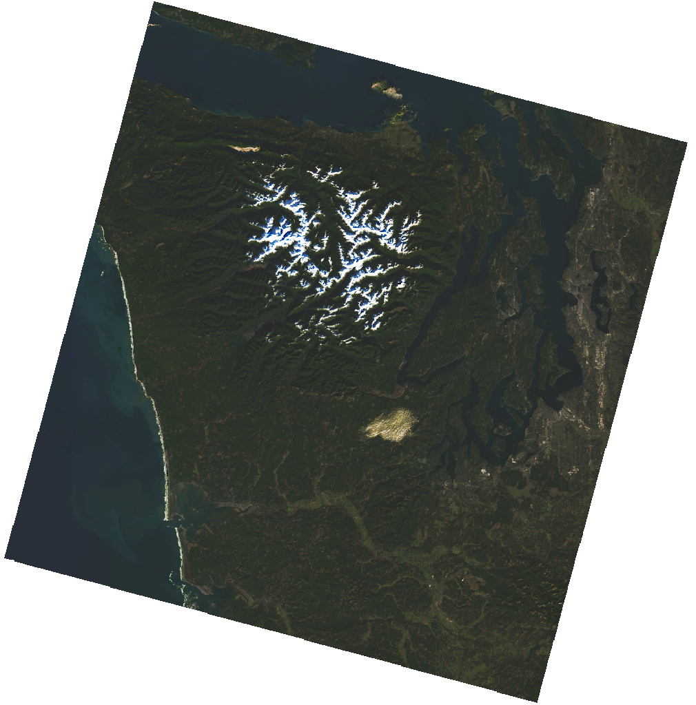
Here, we'll inspect the rendered_preview asset.

In [7]:
selected_item.assets["rendered_preview"].to_dict()
Out[7]:
{'href': 'https://planetarycomputer.microsoft.com/api/data/v1/item/preview.png?collection=landsat-8-c2-l2&item=LC08_L2SP_047027_20201204_02_T1&assets=SR_B4&assets=SR_B3&assets=SR_B2&color_formula=gamma+RGB+2.7%2C+saturation+1.5%2C+sigmoidal+RGB+15+0.55',
 'type': 'image/png',
 'title': 'Rendered preview',
 'rel': 'preview',
 'roles': ['overview']}
In [8]:
from IPython.display import Image

Image(url=selected_item.assets["rendered_preview"].href, width=500)
Out[8]:

That rendered_preview asset is generated dynamically from the raw data using the Planetary Computer's data API. We can access the raw data, stored as Cloud Optimzied GeoTIFFs in Azure Blob Storage, using one of the other assets. That said, we do need to do one more thing before accessing the data. If we simply made a request to the file in blob storage we'd get a 404:

In [9]:
import requests

url = selected_item.assets["SR_B2"].href
print("Accessing", url)
response = requests.get(url)
response
Accessing https://landsateuwest.blob.core.windows.net/landsat-c2/level-2/standard/oli-tirs/2020/047/027/LC08_L2SP_047027_20201204_20210313_02_T1/LC08_L2SP_047027_20201204_20210313_02_T1_SR_B2.TIF
Out[9]:
<Response [404]>

That's because the Plantary Computer uses Azure Blob Storage SAS Tokens to enable access to our data, which allows us to provide the data for free to anyone, anywhere while maintaining some control over the amount of egress for datasets.

To get a token for access, you can use the Planetary Computer's Data Authentication API. You can access that anonymously, or you can provide an API Key for higher rate limits and longer-lived tokens.

You can also use the planetary-computer package to generate tokens and sign asset HREFs for access. You can install via pip with

> pip install planetary-computer
In [10]:
import planetary_computer

# PC_SDK_SUBSCRIPTION_KEY
signed_href = planetary_computer.sign(selected_item).assets["SR_B2"].href

We can load up that single COG using libraries like rioxarray or rasterio

In [11]:
# import xarray as xr
import rioxarray

ds = rioxarray.open_rasterio(signed_href, overview_level=4).squeeze()
img = ds.plot(cmap="Blues", add_colorbar=False)
img.axes.set_axis_off();

If you wish to work with multiple STAC items as a datacube, you can use libraries like stackstac or odc-stac.

In [12]:
import stackstac

ds = stackstac.stack(planetary_computer.sign(items))
ds
Out[12]:
<xarray.DataArray 'stackstac-6a76bcf3889fe96912bc723182731111' (time: 4,
                                                                band: 19,
                                                                y: 7972,
                                                                x: 11722)>
dask.array<fetch_raster_window, shape=(4, 19, 7972, 11722), dtype=float64, chunksize=(1, 1, 1024, 1024), chunktype=numpy.ndarray>
Coordinates: (12/27)
  * time                         (time) datetime64[ns] 2020-12-04T19:02:11.19...
    id                           (time) <U31 'LC08_L2SP_047027_20201204_02_T1...
  * band                         (band) <U13 'SR_B1' 'SR_B2' ... 'SR_QA_AEROSOL'
  * x                            (x) float64 3.534e+05 3.534e+05 ... 7.05e+05
  * y                            (y) float64 5.374e+06 5.374e+06 ... 5.135e+06
    view:off_nadir               int64 0
    ...                           ...
    title                        (band) <U46 'Coastal/Aerosol Band (B1)' ... ...
    gsd                          (band) float64 30.0 30.0 30.0 ... 30.0 30.0
    common_name                  (band) object 'coastal' 'blue' ... None None
    center_wavelength            (band) object 0.44 0.48 0.56 ... None None None
    full_width_half_max          (band) object 0.02 0.06 0.06 ... None None None
    epsg                         int64 32610
Attributes:
    spec:        RasterSpec(epsg=32610, bounds=(353370.0, 5135070.0, 705030.0...
    crs:         epsg:32610
    transform:   | 30.00, 0.00, 353370.00|\n| 0.00,-30.00, 5374230.00|\n| 0.0...
    resolution:  30.0

Searching on additional properties

Previously, we searched for items by space and time. Because the Planetary Computer's STAC API supports the query parameter, you can search on additional properties on the STAC item.

For example, collections like sentinel-2-l2a and landsat-8-c2-l2 both implement the eo STAC extension and include an eo:cloud_cover property. Use query={"eo:cloud_cover": {"lt": 20}} to return only items that are less than 20% cloudy.

In [13]:
time_range = "2020-12-01/2020-12-31"
bbox = [-122.2751, 47.5469, -121.9613, 47.7458]

search = catalog.search(
    collections=["sentinel-2-l2a"],
    bbox=bbox,
    datetime=time_range,
    query={"eo:cloud_cover": {"lt": 20}},
)
items = search.get_all_items()

Other common uses of the query parameter is to filter a collection down to items of a specific type, For example, the GOES-CMI collection includes images from various when the satellite is in various modes, which produces images of either the Full Disk of the earth, the continental United States, or a mesoscale. You can use goes:image-type to filter down to just the ones you want.

In [14]:
search = catalog.search(
    collections=["goes-cmi"],
    bbox=[-67.2729, 25.6000, -61.7999, 27.5423],
    datetime=["2018-09-11T13:00:00Z", "2018-09-11T15:40:00Z"],
    query={"goes:image-type": {"eq": "MESOSCALE"}},
)

Analyzing STAC Metadata

STAC items are proper GeoJSON Features, and so can be treated as a kind of data on their own.

In [15]:
search = catalog.search(
    collections=["sentinel-2-l2a"],
    bbox=[-124.2751, 45.5469, -110.9613, 47.7458],
    datetime="2020-12-26/2020-12-31",
)
items = search.get_all_items()

df = geopandas.GeoDataFrame.from_features(items.to_dict(), crs="epsg:4326")

df[["geometry", "datetime", "s2:mgrs_tile", "eo:cloud_cover"]].explore(
    column="eo:cloud_cover", style_kwds={"fillOpacity": 0.1}
)
Out[15]:
Make this Notebook Trusted to load map: File -> Trust Notebook

Or we can plot cloudiness of a region over time.

In [16]:
import pandas as pd

search = catalog.search(
    collections=["sentinel-2-l2a"],
    bbox=[-124.2751, 45.5469, -123.9613, 45.7458],
    datetime="2020-01-01/2020-12-31",
)
items = search.get_all_items()
df = geopandas.GeoDataFrame.from_features(items.to_dict())
df["datetime"] = pd.to_datetime(df["datetime"])
In [17]:
ts = df.set_index("datetime").sort_index()["eo:cloud_cover"].rolling(7).mean()
ts.plot(title="eo:cloud-cover (7-scene rolling average)");

Working with STAC Catalogs and Collections

Our catalog is a STAC Catalog that we can crawl or search. The Catalog contains STAC Collections for each dataset we have indexed (which is not the yet the entirity of data hosted by the Planetary Computer).

Collections have information about the STAC Items they contain. For instance, here we look at the Bands available for Landsat 8 Collection 2 Level 2 data:

In [18]:
import pandas as pd

landsat = catalog.get_collection("landsat-8-c2-l2")

pd.DataFrame(landsat.extra_fields["summaries"]["eo:bands"])
Out[18]:
gsd name common_name description center_wavelength full_width_half_max
0 30 SR_B1 coastal coastal 0.44 0.02
1 30 SR_B2 blue visible blue 0.48 0.06
2 30 SR_B3 green visible green 0.56 0.06
3 30 SR_B4 red visible red 0.65 0.04
4 30 SR_B5 nir near-infrared 0.86 0.03
5 30 SR_B6 swir16 short-wave infrared 1.60 0.08
6 30 SR_B7 swir22 short-wave infrared 2.20 0.20
7 100 ST_B10 lwir11 long-wave infrared 10.90 0.80
8 30 ST_TRAD NaN thermal radiance NaN NaN
9 30 ST_URAD NaN upwelled radiance NaN NaN
10 30 ST_ATRAN NaN atmospheric transmission NaN NaN
11 30 ST_CDIST NaN distance to nearest cloud NaN NaN
12 30 ST_DRAD NaN downwelled radiance NaN NaN
13 30 ST_EMIS NaN emissivity NaN NaN
14 30 ST_EMSD NaN emissivity standard deviation NaN NaN

We can see what Assets are available on our item with:

In [19]:
pd.DataFrame.from_dict(landsat.extra_fields["item_assets"], orient="index")[
    ["title", "description", "gsd"]
]
Out[19]:
title description gsd
ANG Angle Coefficients File Collection 2 Level-1 Angle Coefficients File (... NaN
SR_B1 Coastal/Aerosol Band (B1) Collection 2 Level-2 Coastal/Aerosol Band (B1)... 30.0
SR_B2 Blue Band (B2) Collection 2 Level-2 Blue Band (B2) Surface Re... 30.0
SR_B3 Green Band (B3) Collection 2 Level-2 Green Band (B3) Surface R... 30.0
SR_B4 Red Band (B4) Collection 2 Level-2 Red Band (B4) Surface Ref... 30.0
SR_B5 Near Infrared Band 0.8 (B5) Collection 2 Level-2 Near Infrared Band 0.8 (B... 30.0
SR_B6 Short-wave Infrared Band 1.6 (B6) Collection 2 Level-2 Short-wave Infrared Band ... 30.0
SR_B7 Short-wave Infrared Band 2.2 (B7) Collection 2 Level-2 Short-wave Infrared Band ... 30.0
ST_QA Surface Temperature Quality Assessment Band Landsat Collection 2 Level-2 Surface Temperatu... 30.0
ST_B10 Surface Temperature Band (B10) Landsat Collection 2 Level-2 Surface Temperatu... 100.0
MTL.txt Product Metadata File Collection 2 Level-1 Product Metadata File (MTL) NaN
MTL.xml Product Metadata File (xml) Collection 2 Level-1 Product Metadata File (xml) NaN
ST_DRAD Downwelled Radiance Band Landsat Collection 2 Level-2 Downwelled Radian... 30.0
ST_EMIS Emissivity Band Landsat Collection 2 Level-2 Emissivity Band S... 30.0
ST_EMSD Emissivity Standard Deviation Band Landsat Collection 2 Level-2 Emissivity Standa... 30.0
ST_TRAD Thermal Radiance Band Landsat Collection 2 Level-2 Thermal Radiance ... 30.0
ST_URAD Upwelled Radiance Band Landsat Collection 2 Level-2 Upwelled Radiance... 30.0
MTL.json Product Metadata File (json) Collection 2 Level-1 Product Metadata File (json) NaN
QA_PIXEL Pixel Quality Assessment Band Collection 2 Level-1 Pixel Quality Assessment ... 30.0
ST_ATRAN Atmospheric Transmittance Band Landsat Collection 2 Level-2 Atmospheric Trans... 30.0
ST_CDIST Cloud Distance Band Landsat Collection 2 Level-2 Cloud Distance Ba... 30.0
QA_RADSAT Radiometric Saturation Quality Assessment Band Collection 2 Level-1 Radiometric Saturation Qu... 30.0
thumbnail Thumbnail image NaN NaN
SR_QA_AEROSOL Aerosol Quality Analysis Band Collection 2 Level-2 Aerosol Quality Analysis ... 30.0
reduced_resolution_browse Reduced resolution browse image NaN NaN

Some collections, like Daymet include collection-level assets. You can use the .assets property to access those assets.

In [20]:
collection = catalog.get_collection("daymet-daily-na")
collection
Out[20]:
<CollectionClient id=daymet-daily-na>

Just like assets on items, these assets include links to data in Azure Blob Storage.

In [21]:
asset = collection.assets["zarr-https"]
asset
Out[21]:
<Asset href=https://daymeteuwest.blob.core.windows.net/daymet-zarr/daily/na.zarr>
In [22]:
import fsspec
import xarray as xr

store = fsspec.get_mapper(asset.href)
ds = xr.open_zarr(store, **asset.extra_fields["xarray:open_kwargs"])
ds
Out[22]:
<xarray.Dataset>
Dimensions:                  (time: 14965, y: 8075, x: 7814, nv: 2)
Coordinates:
    lat                      (y, x) float32 dask.array<chunksize=(284, 584), meta=np.ndarray>
    lon                      (y, x) float32 dask.array<chunksize=(284, 584), meta=np.ndarray>
  * time                     (time) datetime64[ns] 1980-01-01T12:00:00 ... 20...
  * x                        (x) float32 -4.56e+06 -4.559e+06 ... 3.253e+06
  * y                        (y) float32 4.984e+06 4.983e+06 ... -3.09e+06
Dimensions without coordinates: nv
Data variables:
    dayl                     (time, y, x) float32 dask.array<chunksize=(365, 284, 584), meta=np.ndarray>
    lambert_conformal_conic  int16 ...
    prcp                     (time, y, x) float32 dask.array<chunksize=(365, 284, 584), meta=np.ndarray>
    srad                     (time, y, x) float32 dask.array<chunksize=(365, 284, 584), meta=np.ndarray>
    swe                      (time, y, x) float32 dask.array<chunksize=(365, 284, 584), meta=np.ndarray>
    time_bnds                (time, nv) datetime64[ns] dask.array<chunksize=(365, 2), meta=np.ndarray>
    tmax                     (time, y, x) float32 dask.array<chunksize=(365, 284, 584), meta=np.ndarray>
    tmin                     (time, y, x) float32 dask.array<chunksize=(365, 284, 584), meta=np.ndarray>
    vp                       (time, y, x) float32 dask.array<chunksize=(365, 284, 584), meta=np.ndarray>
    yearday                  (time) int16 dask.array<chunksize=(365,), meta=np.ndarray>
Attributes:
    Conventions:       CF-1.6
    Version_data:      Daymet Data Version 4.0
    Version_software:  Daymet Software Version 4.0
    citation:          Please see http://daymet.ornl.gov/ for current Daymet ...
    references:        Please see http://daymet.ornl.gov/ for current informa...
    source:            Daymet Software Version 4.0
    start_year:        1980